
Python Pandas is the #1 tool inside a Data Engineer or Data Scientist toolbox. It allows you to read/write data from a large variety of file formats; and provides extensive built-in functionality to aggregate, join, filter, and transform dataset with high performance. Pandas is the fastest and easiest tool to extract, transform, and load (ETL) dataset which fit in memory and can be process by a single machine.
This lesson will teach you the basic pandas Data Engineering skills.
Getting Started
Git Project
Please make sure you have python3.7 installed on your system.
Clone the git repo:
git clone https://github.com/turalabs/pandas-intro.git
cd pandas-intro
Jupyter Notebook
To follow the exercises in this lesson we will install and use Jupyter Notebook. Jupyter is a standard Data Science and Data Engineering tool. It makes it very easy to combine both markdown instructions and code on Notebook and share it with other people.
Follow the instructions below to install and run Jupyter Notebook with a virtualenv.
install_jupyter.shFor convenience, we've compiled the installation instructions below into install_jupyter.sh. Run the script to install Jupyter Notebook and Themes.
First let's create a new virtual and activate it:
# navigate to the pandas-intro folder if you haven't already
cd pandas-intro

# install and run a virtualenv
python3.7 -m venv venv
source venv/bin/activate
Install and setup Jupyter Notebook along with Jupyter Themes which will make our notebooks to look much more professional. To setup and install Notebook and Themes run:
Make sure your virtualenv is active, otherwise your notebook will start with your default python3 which may NOT contain pandas and other packages that you will install later.
# install jupyter notebook
pip install jupyterlab
pip install notebook

# install and setup jupyter themes
pip install jupyterthemes

# change default theme and fonts
jt -t onedork -T -tf sourcesans -nf sourcesans -tfs 12
Finish the setup by installing pandas and other packages:
# install pandas
pip install pandas pyarrow pandas-gbq
Start a new notebook:
jupyter notebook
Jupyter will start a new server and display the notebook address in the terminal. Copy and paste the notebook URL into your browser.
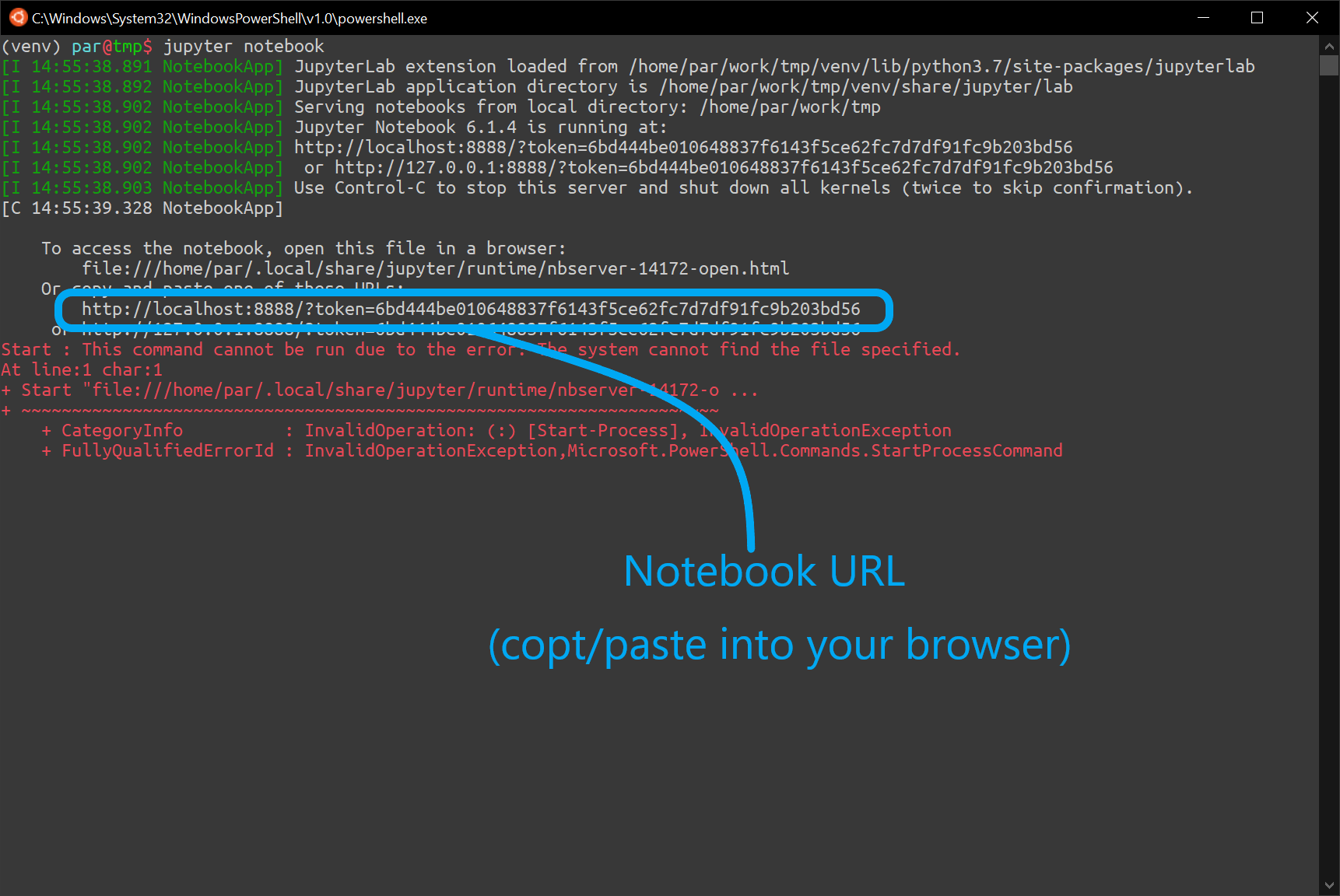
You should be able to browse to the notebooks for this lesson under notebooks folder:
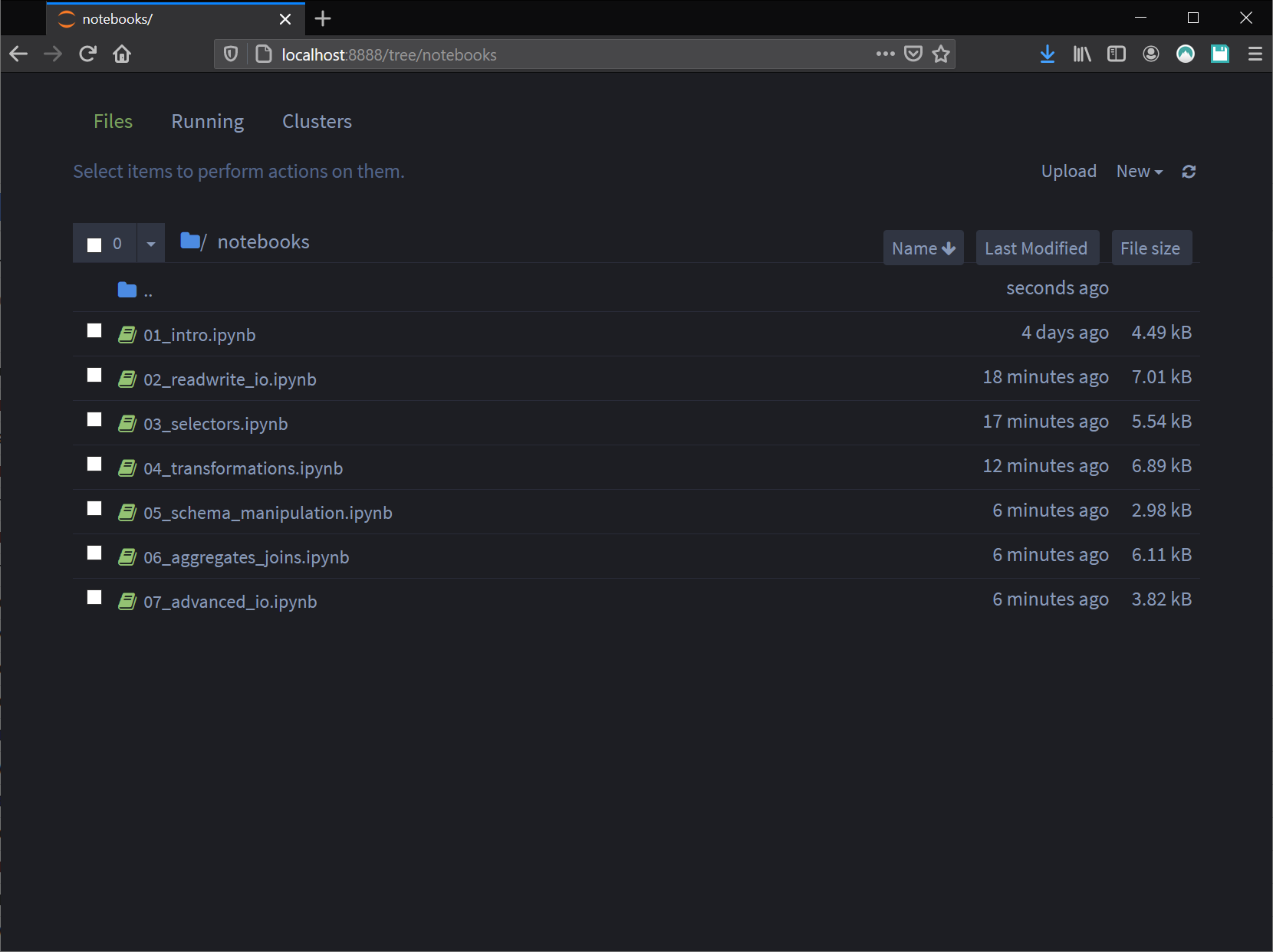
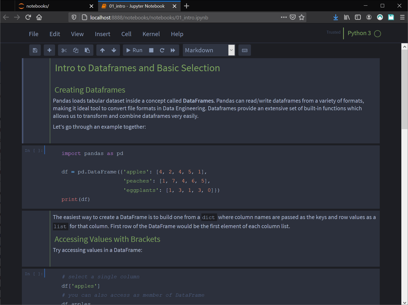
Go ahead and open the first notebook called 01_intro.ipynb for the next section:
You can refer to Jupyter Notebook and Themes Documentation for full setup instructions:
If you see an error when importing pandas from the test notebook, it means that jupyter is using a different ipython kernel than the virtualenv that we installed.
You can either go back to installation steps above and make sure you install and run jupyter from your virtualenv (don't miss the initial instructions for creating and activating a virtualenv).
Alternatively, there's a nice blog post on how to setup different ipython kernels (or virtualenvs) with Jupyter. Follow the instructions here or on the blog post:
python3.7 -m venv pandas-intro
source pandas-intro/bin/activate
pip install ipykernel
ipython kernel install --user --name=pandas-intro
Restart jupyter and switch the notebook kernel from the menu bar: Kernel >> Change kernel >> pandas-intro.
Intro to DataFrames and Basic Selection
Open the jupyter notebook file: 01_intro.ipynb
Creating DataFrames
Pandas loads tabular dataset inside a concept called DataFrames. Pandas can read/write DataFrames from a variety of formats, making it ideal tool to convert file formats in Data Engineering. DataFrames provide an extensive set of built-in functions which allows us to transform and combine DataFrames very easily.
Let's go through an example together:
import pandas as pd

df = pd.DataFrame({'apples': [4, 2, 4, 5, 1],
                   'peaches': [1, 7, 4, 6, 5],
                   'eggplants': [1, 3, 1, 3, 0]})
print(df)
   apples  peaches  eggplants
0       4        1          1
1       2        7          3
2       4        4          1
3       5        6          3
4       1        5          0
The easiest way to create a DataFrame is to build one from a dict where column names are passed as the keys and row values as a list for that column.
First row of the DataFrame would be the first element of each column list.
Accessing Values with Brackets
Try accessing values in a DataFrame:
# select a single column
df['apples']
# access columns as a member of DataFrame
df.apples

# accessing values within a column
df['apples'][0]
df.apples[0]

# access a slice of values
df['apples'][0:2]
[][]When you're using [..][..] to access elements in a DataFrame think of it a a two dimensional array where the first dimension represents the columns and the second dimensions represent the row sequence.
Creating DataFrame with Index
By default pandas assigns a RangeIndex to the rows starting with 0 (similar to lists). This is what we saw in the examples above. However you can specifically assign row labels or indexes for each row:
df = pd.DataFrame({'apples': [4, 2, 4, 5, 1],
                   'peaches': [1, 7, 4, 6, 5],
                   'eggplants': [1, 3, 1, 3, 0]},
                 index=['A', 'B', 'C', 'D', 'E'])
print(df)
   apples  peaches  eggplants
A       4        1          1
B       2        7          3
C       4        4          1
D       5        6          3
E       1        5          0
You can still use brackets to access values:
# you can use both row label (index) by position
# the correct way would be by label
df['apples']['A']
# or by position
df['apples'][0]

# select multiple rows or columns at once
df['apples'][['A', 'E', 'D']]
    A    4
    E    1
    D    5
    Name: apples, dtype: int64
Assigning Values
As easy as reading values, you can also assign values:
# assign a single value
df['apples']['A'] = 10

# assign and add an entire column
df['oranges'] = 0
df['oranges']['D'] = 2


# add an entire row. you will learn .loc() later
df.loc['F'] = {'apples': 3, 'peaches': 0, 'eggplants': 3, 'oranges': 1}

print(df)
   apples  peaches  eggplants  oranges
A      10        1          1        0
B       2        7          3        0
C       4        4          1        0
D       5        6          3        2
E       1        5          0        0
F       3        0          3        1
I/O: Reading and Writing Data
Open the jupyter notebook file: 02_readwrite_io.ipynb
The most standard use of pandas is to read and write data files. Pandas provides a series of built-in I/O functions to read and write data from various files formats; making it the defacto standard tool to convert files formats.
Pandas is often used to read data from basic internet and SQL files formats such as CSVs and Json files and transform them into Big Data formats such as Parguet, ORC, BigQuery, and other formats.
Reading CSV
Amongst pandas built-in readers you can use read_csv to import data from
a delimited file:
flights.csv Data files for this lesson are included under data/ forlder. The flights.csv files contains all domestic (USA) flights for 2019 Thanksgiving Day.
These are real flight records from United States Bureau of Transportation.
import pandas as pd

flights = pd.read_csv('../data/flights.csv', header=0)
print(flights.head())
  flight_date airline tailnumber  flight_number  src dest  departure_time   arrival_time  flight_time  distance
0  2019-11-28      9E     N8974C           3280  CHA  DTW            1300           1455        115.0     505.0
1  2019-11-28      9E     N901XJ           3281  JAX  RDU             700            824         84.0     407.0
2  2019-11-28      9E     N901XJ           3282  RDU  LGA             900           1039         99.0     431.0
3  2019-11-28      9E     N912XJ           3283  DTW  ATW            1216           1242         86.0     296.0
4  2019-11-28      9E     N924XJ           3284  DSM  MSP            1103           1211         68.0     232.0
read_csv methods provides a series of options to parse csv files correctly. The header option is used to extract column names
from a csv header row. header=0 marks the first row of csv (row 0) as the header row.
Feel free to set other options:
import pandas as pd

# setting separator and line terminator characters
flights = pd.read_csv('../data/flights.csv', header=0, sep=',', lineterminator='\n')

# reading only 10 rows and selected columns
flights = pd.read_csv('../data/flights.csv', header=0, nrows=10,
                      usecols=['airline', 'src', 'dest'])
print(flights.head())
read_csv optionsFor the full list of available read_csv options refer to the online
documentation
Assigning data types
You can set column data types using the dtype option:
import pandas as pd
import numpy as np

# using `dtype` to assign particular column data types
flights = pd.read_csv('../data/flights.csv', header=0,
                      dtype={
                          'flight_time': np.int16,
                          'distance': np.int16
                      })

# print
print(flights.head(10))
    flight_date airline tailnumber  flight_number  src dest  departure_time  arrival_time  flight_time  distance
0  2019-11-28      9E     N8974C           3280  CHA  DTW            1300          1455          115       505
1  2019-11-28      9E     N901XJ           3281  JAX  RDU             700           824           84       407
2  2019-11-28      9E     N901XJ           3282  RDU  LGA             900          1039           99       431
3  2019-11-28      9E     N912XJ           3283  DTW  ATW            1216          1242           86       296
4  2019-11-28      9E     N924XJ           3284  DSM  MSP            1103          1211           68       232
5  2019-11-28      9E     N833AY           3285  LGA  PWM            1013          1144           91       269
6  2019-11-28      9E     N314PQ           3286  CLE  DTW            1400          1502           62        95
7  2019-11-28      9E     N686BR           3288  DTW  LAN            1227          1314           47        74
8  2019-11-28      9E     N686BR           3288  LAN  DTW            1350          1440           50        74
9  2019-11-28      9E     N147PQ           3289  JFK  ROC            2100          2233           93       264
Data types are typically set as numpy types. The dtype parameter is specifically handy since it allows you to set specific columns and leave the rest for pandas to figure out.
Using Converters
The most convenient way to parse special columns and apply business rules to transform fields at ingest is using the converters option of read_csv.
You can use specific function to parse special fields. In this case we use a couple functions called decode_flightdate and decode_tailnumber to parse flight dates and drop the initial letter 'N' from tailnumber. We also show that you can use lambda functions as converters:
import pandas as pd
from datetime import datetime

def decode_flightdate(value:str):
    try:
        return datetime.strptime(value, '%Y-%m-%d').date()
    except (ValueError, TypeError):
        return None

def decode_tailnumber(value:str):
    if str(value).startswith('N'):
        return str(value)[1:]
    else:
        return str(value)

# using `converters` to pass functions to parse fields
flights = pd.read_csv('../data/flights.csv', header=0,
                      converters={
                          'flight_time': decode_flightdate,
                          'tailnumber': decode_tailnumber,
                          'flight_time': (lambda v: int(float(v))),
                          'distance': (lambda v: int(float(v))),
                      })

# print
print(flights.head(10))
    flight_date airline tailnumber  flight_number  src dest  departure_time  arrival_time  flight_time  distance
0  2019-11-28      9E      8974C           3280  CHA  DTW            1300          1455          115       505
1  2019-11-28      9E      901XJ           3281  JAX  RDU             700           824           84       407
2  2019-11-28      9E      901XJ           3282  RDU  LGA             900          1039           99       431
3  2019-11-28      9E      912XJ           3283  DTW  ATW            1216          1242           86       296
4  2019-11-28      9E      924XJ           3284  DSM  MSP            1103          1211           68       232
5  2019-11-28      9E      833AY           3285  LGA  PWM            1013          1144           91       269
6  2019-11-28      9E      314PQ           3286  CLE  DTW            1400          1502           62        95
7  2019-11-28      9E      686BR           3288  DTW  LAN            1227          1314           47        74
8  2019-11-28      9E      686BR           3288  LAN  DTW            1350          1440           50        74
9  2019-11-28      9E      147PQ           3289  JFK  ROC            2100          2233           93       264
converters functionsWe highly recommend using the converter functions for parsing and applying business rules and cleansing rules at parse time with read_csv.
Writing Data
Pandas provides a series of I/O write functions. You can read the documentation to use appropriate function for your use-case.
Here we're going to write our flights into both Json Row and Parquet formats:
import pandas as pd

# read csv
flights = pd.read_csv('../data/flights.csv', header=0)

# write json row format
flights.to_json('../data/flights.json', orient='records', lines=True)
# write compressed parquet format
flights.to_parquet('../data/flights.parquet', engine='pyarrow',
                   compression='gzip', index=False)
head data/flights.json
{"flight_date":"2019-11-28","airline":"9E","tailnumber":"N8974C","flight_number":3280,"src":"CHA","dest":"DTW","departure_time":1300,"arrival_time":1455,"flight_time":115.0,"distance":505.0}
{"flight_date":"2019-11-28","airline":"9E","tailnumber":"N901XJ","flight_number":3281,"src":"JAX","dest":"RDU","departure_time":700,"arrival_time":824,"flight_time":84.0,"distance":407.0}
{"flight_date":"2019-11-28","airline":"9E","tailnumber":"N901XJ","flight_number":3282,"src":"RDU","dest":"LGA","departure_time":900,"arrival_time":1039,"flight_time":99.0,"distance":431.0}
{"flight_date":"2019-11-28","airline":"9E","tailnumber":"N912XJ","flight_number":3283,"src":"DTW","dest":"ATW","departure_time":1216,"arrival_time":1242,"flight_time":86.0,"distance":296.0}
{"flight_date":"2019-11-28","airline":"9E","tailnumber":"N924XJ","flight_number":3284,"src":"DSM","dest":"MSP","departure_time":1103,"arrival_time":1211,"flight_time":68.0,"distance":232.0}
{"flight_date":"2019-11-28","airline":"9E","tailnumber":"N833AY","flight_number":3285,"src":"LGA","dest":"PWM","departure_time":1013,"arrival_time":1144,"flight_time":91.0,"distance":269.0}
{"flight_date":"2019-11-28","airline":"9E","tailnumber":"N314PQ","flight_number":3286,"src":"CLE","dest":"DTW","departure_time":1400,"arrival_time":1502,"flight_time":62.0,"distance":95.0}
{"flight_date":"2019-11-28","airline":"9E","tailnumber":"N686BR","flight_number":3288,"src":"DTW","dest":"LAN","departure_time":1227,"arrival_time":1314,"flight_time":47.0,"distance":74.0}
{"flight_date":"2019-11-28","airline":"9E","tailnumber":"N686BR","flight_number":3288,"src":"LAN","dest":"DTW","departure_time":1350,"arrival_time":1440,"flight_time":50.0,"distance":74.0}
{"flight_date":"2019-11-28","airline":"9E","tailnumber":"N147PQ","flight_number":3289,"src":"JFK","dest":"ROC","departure_time":2100,"arrival_time":2233,"flight_time":93.0,"distance":264.0}
Advanced Selectors
Open the jupyter notebook file: 03_selectors.ipynb
Selecting with .loc and .iloc
Aside from using double brackets [][] to access values, DataFrame provides .loc[] and 'iloc[] mthods to select values with row labels (index) or position respectively.
Here's some examples of using .loc()
import pandas as pd

# read data fom csv
flights = pd.read_csv('../data/flights.csv', header=0)

# select single row by index
flights.loc[0]

# select multiple rows with slices
flights.loc[[0, 5, 7, 10]]
flights.loc[0:3]

# select multiple rows and columns by index
flights.loc[0:3,['airline', 'src', 'dest']]
.loc[[rows],[columns]]Using .loc the first bracket selects rows and the second bracket select column. This is the reverse order of using double brackets.
.iloc[] works the same way, but instead of labels (index) you can select by row and colunm position numbers. In this case, since our flight records have a RangeIndex the row indexes are the same as labels:
# select first row
flights.iloc[0]

# select multiple rows with slices
flights.iloc[[0, 5, 7, 10]]
flights.iloc[0:3]

# select multiple rows and columns by position
flights.iloc[0:3,[0, 2, 4]]
.loc and ilocYou can always mix using .loc and iloc together:
# mixing loc and iloc
# select rows 5-10 and few columns
flights.iloc[5:10].loc[:, ['flight_number', 'src', 'dest']]
Conditional Selections
You can specify criteria for selecting values within the DataFrame:
# select delta airline flights
flights.loc[flights.airline == 'DL']
# same as above
flights.loc[flights['airline'] == 'DL']

# flights where distance is not null
flights.loc[flights.distance.notna()]
# or where distance is null
flights.loc[flights.distance.isna()]

# select flights out of PDX over 500 miles
flights.loc[(flights.src == 'PDX') & (flights.distance > 500.0)]

# apply multiple conditions::
# select delta or alaska flights
flights.loc[(flights.airline == 'DL') | (flights.airline == 'AS')]
# select delta airlines flights from LAX-JFK
flights.loc[(flights.airline == 'DL') & (flights.src == 'LAX') & (flights.dest == 'JFK')]

# select delta and alaska flights from LAX-JSK
flights.loc[flights.airline.isin(['DL', 'AS']) &
            (flights.src == 'LAX') & (flights.dest == 'JFK')]
     flight_date airline tailnumber  flight_number  src dest  departure_time  arrival_time  flight_time  distance
2006  2019-11-28      AS     N238AK            410  LAX  JFK             700          1530        330.0    2475.0
2024  2019-11-28      AS     N282AK            452  LAX  JFK            1040          1909        329.0    2475.0
2028  2019-11-28      AS     N461AS            460  LAX  JFK            2325           748        323.0    2475.0
2035  2019-11-28      AS     N266AK            470  LAX  JFK            2035           500        325.0    2475.0
3395  2019-11-28      DL     N177DN           1436  LAX  JFK             605          1425        320.0    2475.0
3815  2019-11-28      DL     N179DN           2164  LAX  JFK             915          1742        327.0    2475.0
4174  2019-11-28      DL     N195DN           2815  LAX  JFK            2100           516        316.0    2475.0
4521  2019-11-28      DL     N183DN            816  LAX  JFK            1115          1949        334.0    2475.0
Pandas has special selections method for almost everything. Remember them and use them rigorously. Methods such as .isin(), .isna(), and .notna(). See examples above.
Using query() method
If you are more familiar with SQL syntax, you can use the pandas .query() method:
# select flights from PDX over 500 miles
flights.query("(src == 'PDX') & (distance > 500.0)")
Subselections
You can always save a selection and further subselect within a set by assigning your selections into a variable:
# select flights from PDX
pdx_flights = flights.loc[flights.src == 'PDX']
# find long distance flights
pdx_long_distance = pdx_flights.query("distance > 500.0")
pdx_long_distance
Transformations
Open the jupyter notebook file: 04_transformations.ipynb
Map()
Pandas comes very handy when it comes to applying transformation rules to columns. The simplest method is to apply a map() function to transform values within a a column:
import pandas as pd

# read data fom csv
flights = pd.read_csv('../data/flights.csv', header=0)

def decode_airline(value:str):
    mapper = {
        'AA': 'American Airlines',
        'AS': 'Alaska Airlines',
        'DL': 'Delta Air Lines',
        'UA': 'United Airlines',
        'WN': 'Southwest Airlines',
    }
    if value in mapper:
        return mapper[value]
    else:
        return 'Other'

# decode airline names and assign to a new column
flights['airline_name'] = flights.airline.map(decode_airline)

# print decoded flights
flights.loc[flights.airline_name != 'Other'][['airline', 'airline_name', 'src', 'dest']]
    airline       airline_name  src dest
299      AA  American Airlines  PHX  ORD
300      AA  American Airlines  ORD  DCA
301      AA  American Airlines  STL  ORD
302      AA  American Airlines  SFO  DFW
303      AA  American Airlines  CLT  PBI
304      AA  American Airlines  DFW  SLC
305      AA  American Airlines  DFW  BNA
306      AA  American Airlines  DFW  IND
307      AA  American Airlines  SJC  DFW
308      AA  American Airlines  HNL  DFW
Let's practice more to get familiar with using map() effectively:
from datetime import datetime, date

def decode_flightdate(value):
    # check if value is already a date instance? parse as date if not
    if isinstance(value, date):
        return value
    else:
        return datetime.strptime(value, '%Y-%m-%d').date()

# re-assign flight_date as datetime
flights.flight_date = flights.flight_date.map(decode_flightdate)

# use lambda functions as map
flights.distance = flights.distance.map(lambda v: int(v))

print(flights.head(5))
Apply()
While the .map() method allows transformation over a single column, pandas DataFrame .apply() method allows transformation over multiple column values. You can use .apply() when you need to transform more than one column within a row.
For example encode_flight_key method concatenates airline, flight_number, src, and dest fields to create a unique flight key for each row:
import pandas as pd

# read data fom csv
flights = pd.read_csv('../data/flights.csv', header=0)

def encode_flight_key(row):
    # a dataframe row is passed. access columns with row.column_name
    flight_key = f"{row.airline}{row.flight_number}-{row.src}-{row.dest}"
    return flight_key

# apply a function over entire row values
# set axis=1 to apply function over rows. axis=0 would apply over columns
flights['flight_key'] = flights.apply(encode_flight_key, axis=1)
flights['flight_key']
0        9E3280-CHA-DTW
1        9E3281-JAX-RDU
2        9E3282-RDU-LGA
3        9E3283-DTW-ATW
4        9E3284-DSM-MSP
                ...
12710    YX6119-CMH-LGA
12711    YX6120-IND-LGA
12712    YX6122-DCA-BOS
12713    YX6139-BOS-ORD
12714    YX6139-ORD-BOS
Name: flight_key, Length: 12715, dtype: object
Pay attention to axis=1 which directs pandas to apply the function horizontally over row values. axis=0 directs pandas to apply a function vertically to all column values. Please refer to DataFrame.apply documentation for more information.
Pandas passes the row values as the first parameter to the apply function. You can use the args parameter if your function requires more parameters. For example:
# passing more parameters to apply function by position
def encode_flight_key(row, key_type):
    # a dataframe row is passed. access columns with row.column_name
    if key_type == "short":
        flight_key = f"{row.airline}{row.flight_number}-{row.src}-{row.dest}"
    else:
        flight_key = f"{row.flight_date}-{row.airline}{row.flight_number}-{row.src}-{row.dest}"
    return flight_key

# apply a function over entire row values
# pass additional positional parameters to apply function
flights['flight_key'] = flights.apply(encode_flight_key, axis=1, args=("short",))
flights['flight_key_long'] = flights.apply(encode_flight_key, axis=1, args=("long",))

# print
flights[['flight_key', 'flight_key_long']]
Complex
The section below shows an example where we apply a function over multiple columns which produces multiple columns in a DataFrame.
In this example, we will produce two new columns called "is_commuter" and "is_long_distance" depending on flight's duration and distance.
def encode_flight_type(row):
    # commuter: distance less than 300 miles and flight time less than 90 mins
    # long distance: distance greater than 1500 miles and flight time over 3 hours
    is_commuter = row.distance < 300.0 and row.flight_time < 90.0
    is_long_distance = row.distance > 1500.0 and row.flight_time > 180.0
    # return a tuple
    return (is_commuter, is_long_distance)

# apply a function over row values and
# unpack multiple return column values by using zip()
flights['is_commuter'], flights['is_long_distance'] = zip(*flights.apply(
                                                        encode_flight_type, axis=1))

# print
flights.loc[flights.is_commuter == True]
Schema Manipulation
Open the jupyter notebook file: 05_schema_manipulation.ipynb
Renaming and Dropping
You often need to rename or drop columns. Further you might also want to remove rows from your DataFrame. The example below shows you how to do this:
import pandas as pd

# read data fom csv
flights = pd.read_csv('../data/flights.csv', header=0)

# rename dataframe column
flights.rename(columns={'flight_date': 'fdate',
                        'flight_number': 'fnum',
                        'tailnumber': 'tailnum'}, inplace=True, errors='ignore')

# drop columns
flights.drop(columns=['flight_time', 'distance'], inplace=True, errors='ignore')

# remove rows - removing rows 0-3 by their label (index)
flights.drop(labels=[0,1,2], inplace=True, errors='ignore')
Set and Reset Index
You can always set and reset the index column in a DataFrame. Pandas provides a series of methods to do this. The most common method is to use the .set_index() method:
import pandas as pd

# read data fom csv
flights = pd.read_csv('../data/flights.csv', header=0)

# create a flight_key column by concatenating airline, flight_number, src, and dest
flights['flight_key'] = flights.apply(
    (lambda r: f"{r.airline}{r.flight_number}-{r.src}-{r.dest}"),
     axis=1)

# set the index to the new flight_key column
flights.set_index(keys=['flight_key'], inplace=True)

# print flight 6122 DCA to BOS
flights.loc['YX6122-DCA-BOS']
flight_date       2019-11-28
airline                   YX
tailnumber            N211JQ
flight_number           6122
src                      DCA
dest                     BOS
departure_time           900
arrival_time            1038
flight_time               98
distance                 399
Name: YX6122-DCA-BOS, dtype: object
You can reset index columns back into the DataFrame by using the .reset_index() method:
# you can reset indexed columns back into the dataframe by:
flights.reset_index(inplace=True)
flights
Aggregates and Joins
Open the jupyter notebook file: 06_aggregates_joins.ipynb
Summary Methods
Pandas provides a series of very helpful summary functions. These functions provide easy and quick overview of data inside the DataFrame. We can easily get things like counts, mean values, unique counts, and frequency of values:
import pandas as pd

# read data fom csv
flights = pd.read_csv('../data/flights.csv', header=0)

# invoke summary methods on columns
# describe method on a text field
flights.src.describe()
# describe method on float field
flights.flight_time.describe()

# getting unique values
flights.airline.unique()
count    12715.000000
mean       146.176956
std         75.611148
min         34.000000
25%         90.000000
50%        128.000000
75%        175.000000
max        675.000000
Name: flight_time, dtype: float64

array(['9E', 'AA', 'AS', 'B6', 'DL', 'EV', 'F9', 'G4', 'HA', 'MQ', 'NK',
       'OH', 'OO', 'UA', 'WN', 'YV', 'YX'], dtype=object)
Aggregates
Pandas provides a .groupby() method which makes it easy to compute aggregates over the DataFrame. This is very handy to find things like sums, counts, min. and max values.
The example below shows how to use count(), sum(), min(), and max():
import pandas as pd

# read data fom csv
flights = pd.read_csv('../data/flights.csv', header=0)

# get flight counts by airline
flights_per_airline = flights.groupby('airline').flight_number.count()

# total traveled miles by airlines
miles_per_airline = flights.groupby('airline').distance.sum()
# use other functions like min, max with aggregates
min_distance_per_airlines = flights.groupby('airline').distance.min()
max_distance_per_airlines = flights.groupby('airline').distance.max()

print("flights per airline:\n", flights_per_airline.head(5))
print("miles per airline:\n", miles_per_airline.head(5))
print("min distance per airline:\n", min_distance_per_airlines.head(5))
print("max distance per airline:\n", max_distance_per_airlines.head(5))
flights per airline:
    airline
9E     299
AA    1379
AS     642
B6     802
DL    1514
Name: flight_number, dtype: int64
miles per airline:
    airline
9E     120270.0
AA    1392336.0
AS     875079.0
B6     916665.0
DL    1260869.0
Name: distance, dtype: float64
min distance per airline:
    airline
9E    74.0
AA    84.0
AS    95.0
B6    68.0
DL    95.0
Name: distance, dtype: float64
max distance per airline:
    airline
9E    1107.0
AA    4243.0
AS    2846.0
B6    2704.0
DL    4502.0
Name: distance, dtype: float64
Multiple Aggregates Stitched Together
The example below shows how you can create a grouped (aggregated) series to compute different aggregate on multiple columns, or even apply a transformation, and then stitched everything back to display the results.
The key here is that pandas creates an indexed series when you use a .groupby() method. The index is set to the group keys used for any consequent aggregates:
# create a grouped series
grouped = flights.groupby('airline')
# create aggregates series
flight_count = grouped.flight_number.count()
total_distance = grouped.distance.sum()
min_distance = grouped.distance.min()
max_distance = grouped.distance.max()
# change series names
counts.name,  total_distance.name = 'flight_count', 'total_distance'
min_distance.name, max_distance.name = 'min_dist', 'max_dist'
# stitch back the aggregated together
stitched_back = pd.concat([flight_count, total_distance, min_distance, max_distance], axis=1)

# print
print(stitched_back.head(5))
            flight_count  total_distance  min_dist  max_dist
airline
9E                299        120270.0      74.0    1107.0
AA               1379       1392336.0      84.0    4243.0
AS                642        875079.0      95.0    2846.0
B6                802        916665.0      68.0    2704.0
DL               1514       1260869.0      95.0    4502.0
Multiple Aggregates Using .aggr()
Alternatively, pandas provides the .agg() method to apply multiple aggregates on a column at the same time. You can accomplished the same results much more concisely by using the .agg() method such as:
# create a grouped series
grouped = flights.groupby('airline').distance.agg([len, sum, min, max])
print(grouped.head(5))
            len        sum   min     max
airline
9E        299.0   120270.0  74.0  1107.0
AA       1379.0  1392336.0  84.0  4243.0
AS        642.0   875079.0  95.0  2846.0
B6        802.0   916665.0  68.0  2704.0
DL       1514.0  1260869.0  95.0  4502.0
GroupBy Multiple Columns
You can pass an array of columns to groupby() method to aggregate by multiple columns at the same time. The example below calculates flight counts per airline route (airline, src, dest):
# get flight counts for distinct routes
flights_per_route = flights.groupby(['airline', 'src', 'dest']).flight_number.count()
flights_per_route
airline  src  dest
9E       AEX  ATL     1
         AGS  ATL     4
         ATL  ABE     1
              AEX     1
              AGS     4
                     ..
YX       TYS  LGA     1
              MIA     1
         XNA  CLT     1
              IAH     1
              LGA     1
Name: flight_number, Length: 6971, dtype: int64
Sorting Values
Use the .sort_values() series method to sort a DataFrame based on values of a column:
# get total flight distance by airline
grouped = flights.groupby('airline').distance.sum()
# sort in descending order
grouped.sort_values(ascending=False)
airline
WN    1842840.0
AA    1392336.0
UA    1342572.0
DL    1260869.0
B6     916665.0
AS     875079.0
NK     605935.0
OO     603012.0
F9     403572.0
YX     282498.0
YV     214806.0
MQ     186974.0
HA     176718.0
OH     153678.0
G4     133766.0
9E     120270.0
EV     117090.0
Name: distance, dtype: float64
Advanced Read/Write IO
Open the jupyter notebook file: 07_advanced_io.ipynb
Pandas provides built-in methods to read/write to almost every prominent Big Data file and storage type; making pandas one of the standard tools for converting data formats and loading data.
Writing to Cloud BigQuery
One of the key applications of pandas is to transform data files and load into Big Data / Cloud tools for analytics. Pandas provides a built-in method called .to_gbq() to load DataFrames into BigQuery.
The example below shows how you can use the .to_gbq() method to load data into BigQuery.
Use .to_gbq() on smaller data loads (typically less than 1GB). The underlying method used by this method is not meant for large data loads. We recommend using this method for data loads in MBs range. Other techniques like writing directly to GCS and using BigQuery external tables is preferred method for large data loads in GB range.
import pandas as pd
from google.oauth2 import service_account
import os

# read data fom csv
flights = pd.read_csv('../data/flights.csv', header=0)

# check if GCP credentials file is set
if os.getenv('GOOGLE_APPLICATION_CREDENTIALS', default=None) is None:
    raise RuntimeError("You forgot to set GOOGLE_APPLICATION_CREDENTIALS environment variable!")

# you can explicitly load google credentials from a service account json file
# this is OPTIONAL if GOOGLE_APPLICATION_CREDENTIALS environment variable is set
credentials = service_account.Credentials.from_service_account_file(
                    os.getenv('GOOGLE_APPLICATION_CREDENTIALS'))

# schema is used to map DataFrame fields to BigQuery data types
# field data types should be defined as: https://cloud.google.com/bigquery/docs/schemasqbg_df
schema = [
    {'name': 'airline', 'type': 'STRING'},
    {'name': 'src', 'type': 'STRING'},
    {'name': 'dest', 'type': 'STRING'},
    {'name': 'flight_number', 'type': 'STRING'},
    {'name': 'departure_time', 'type': 'STRING'},
    {'name': 'arrival_time', 'type': 'STRING'},
]
# gcp project name, bigquery dataset and tables names
# EDIT values below based on your GCP environment
project = 'deb-airliner'
dataset = 'airline_data'
table = 'pandas_flights'
# filter output dataframe
qbg_df = flights[['airline', 'src', 'dest',
                  'flight_number', 'departure_time', 'arrival_time']]
# write to bigquery using .to_gbq()
qbg_df.to_gbq(
    destination_table=f"{dataset}.{table}",
    project_id=project,
    chunksize= 2000,
    if_exists='replace',
    table_schema=schema,
    progress_bar=False,
    credentials=credentials,
)

print('done')
Conclusion
Python pandas is great tool for reading, transforming, and writing data files. Over the years pandas has become the #1 tool used by Data Engineers and Data Scientist. Learning to use pandas can greatly improve your abilities as a Data Engineer.
After going through the exercises in this intro, please feel free to refer to Pandas Documentation for specific help on using particular methods
Another good resource is the Kaggle Course on Pandas. Most concept in their course is covered here; but feel free to reinforce your learning with their course.
Pandas Documentation also has a great 10 minutes to Pandas intro.
Updated on: 2020.09.28